


What is an absolute encoder
Absolute encoders exist in different variants but there are two main families
- Absolute single-turn encoders
- Absolute multiturn encoders
General
Absolute encoders are, like incremental encoders, automation components whose main function is to provide a signal, or rather an absolute code, to a central unit (computer, programmable controller, etc.) in order to be able to position an angular or linear axis.
What is the difference between an incremental encoder and an absolute encoder?
In terms of the mechanical interface, there are practically none, apart from the dimensions for the absolute multiturn encoders (there are still a number of additional components to count the number of turns according to the technology used). All current manufacturers are striving to develop absolute encoders with the same dimensions as incremental encoders.
In terms of the electronic interface, everything changes. An absolute encoder generates a code on x bits according to its angular position and according to n turns for multiturns encoders.
The remarkable difference between an incremental encoder and an absolute encoder is in the process management of the machine automation. Unlike the incremental encoder, the absolute encoder does not require, during power-up, a cycle for referencing the different axes of a machine. When a machine equipped with absolute encoders is energized, it is immediately ready to produce whatever the mechanical position of its axes. This saves precious time when starting up a production unit.
Single-turn absolute encoders
As their name suggests, they only provide angular information on 360 mechanical degrees
- In magnetic technology
- In optical technology (the most common)
- In inductive technology
Whatever the technology used, they provide an absolute code which will be processed by an automaton or a computer (processing unit).
The absolute encoder is mechanically integral with the drive axis (motor; machine tool axes; cable sensors; Robots etc.)
The output codes can be in parallel, in series, or in Fieldbus.
The parallel code
The GRAY code, also called Reflected Binary (RB) or Reflected Binary Code (RBC)
It is the most common code in parallel connection because it has an undeniable advantage over binary code and BCD.
In the late 1940s, the physicist Frank Gray, employed in BELL’s R&D department, was faced with a problem of coding reliability. On 03/17/1953, the company BELL TELEPHONE LABOR INC filed the patent US2632058A of which Frank Gray is designated as inventor.
The peculiarity of the GRAY code is that 1 single bit changes at each state regardless of the number of bits delivered by the encoder, unlike pure binary code where when the most significant bit changes state, n least significant bits change also state.
(See table below).
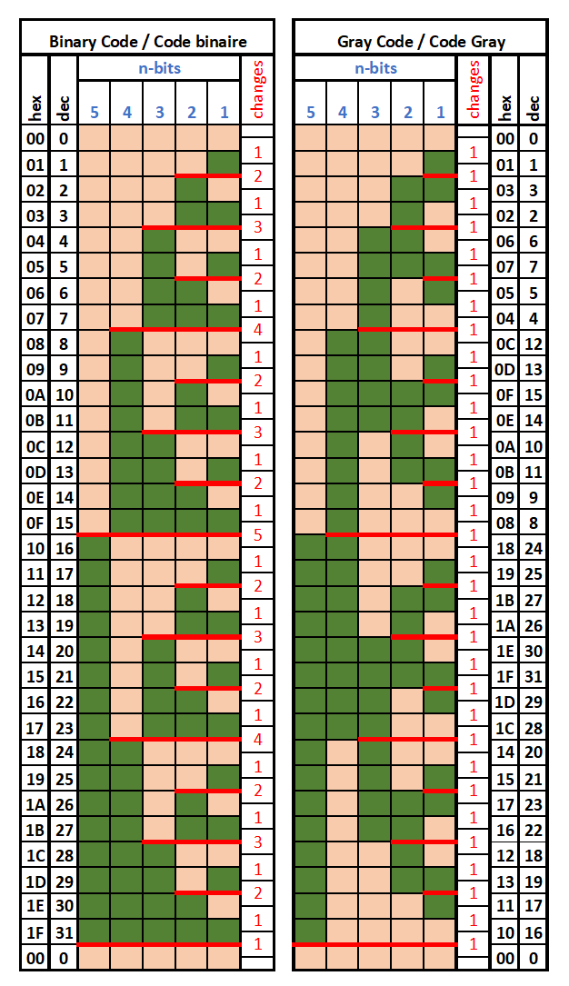
Binary code
On the diagram above we can clearly see this drawback. Passing from the decimal value 0 to the value 31 we see that 5 bits change state at the same time which is a very important problem with an angular encoder. Machine vibrations and more or less jitter can lead to very large reading errors. This is the main reason for the gradual abandonment of the Binary code in the manufacturing of absolute angular encoders with parallel output. To overcome this defect, the binary absolute encoders were often proposed with an additional signal called LATCH and which made it possible to read the code without ambiguity.
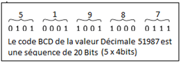
BCD code
This is the binary code encoded in decimal.
During the 1960s and 1970s, some encoder manufacturers manufactured made encoders with an output code in BCD. This code was very practical and especially used with position displays with NIXIES tubes on DIVISIONS (position control system) as for example in sawmills.
An example of BCD code below:
The serial code, also called Synchronous Serial Interface
The parallel codes are certainly very fast. But the lengths of cables between the sensor and the acquisition system are limited to around thirty meters.
But the SSI link has an undeniable cost advantage.
Regardless of the number of bits to be transmitted, a cable of 6 conductors (2 for the clock; 2 for the data and 2 for the power supply) is sufficient whereas for the parallel link, 26 conductors (typically 24 for the data and 2 for the power supply).
Unfortunately the SSI does not allow any dialogue between the encoder and the PLC. The transmission is unidirectional, ie only in the direction of the encoder towards the PLC. It is therefore not possible to monitor the correct functioning of the encoder, such as for example the temperature, the frequency, the logic levels of the signals, etc.
It is to overcome these drawbacks that we have developed fieldbuses.
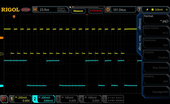
Below is an example of a SSI frame, read on a screen :
Fieldbuses
Generalities
The bus is the abbreviation for “Binary Unit System”. This system is used within a network for the transmission of data between encoders (sensors) and actuators. This data exchange takes place via a common transmission path, but the individual data transmissions are clearly separated from each other.
Fieldbus systems created in the 1980s are essential in the industry today. As an integral part of complex machines and systems, they are mainly used in production automation. But the fieldbus is also used in building automation (home automation) as well as in automotive technology.
Using the field bus online and in series, sensors (encoders; proximity switches; photoelectric cells, etc.) and actuators (solenoid valves; relays; motor contactor, etc.) are connected to programmable logic controllers (API) or also Industrial Programmable Logic and control and processing computers. The fieldbus therefore supports the rapid exchange of data between the various components of the system, even over long distances. Since the fieldbus only communicates via a single cable, the wiring effort has been considerably reduced compared to the wiring of parallel sensors and encoders. A fieldbus operates in so-called “master-slave mode”. While the master is responsible for controlling the processes, the slave stations process the individual subtasks.
Advantages of the fieldbus
Efficiency: Thanks to reduced wiring (only one cable), the start-up times for installations and machines are shortened
Reliability: The reliability of communications between sensors and the central unit is increased thanks to a wiring reduced to the minimum. Short links increase both the availability and reliability of systems.
Immunity to electromagnetic noise: in particular with analog values, fieldbuses offer increased protection against electromagnetic noise.
Uniformity: Thanks to standardized bus protocols and standardized connection technology, encoders from different manufacturers can be used and interchanged more easily. This means that all the individual components do not necessarily have to come from the same manufacturer and it also facilitates the supply in case of urgent maintenance in a shutdown factory due to a faulty encoder.
Flexibility: Even system and machine extensions and modifications can be carried out quickly and easily with fieldbuses. In this way, systems can be variably adapted to new requirements and reused to improve the performance of machines and systems.
Disadvantages of the fieldbus
Complexity: As a fieldbus is a complex system, highly qualified personnel are necessary for the start-up and maintenance of the installations.
Cost: The individual automation components of the fieldbus are much more expensive
Danger: in the event of a bus failure, the control system may be cut off from the sensors, encoders and actuators. To avoid this, redundant bus systems can be installed if necessary.
Response time: longer compared to parallel interfaces.
Most used fieldbuses
There are currently a multitude of fieldbuses such as:
BISS Interface; CANopen; DeviceNet; EtherCAT; EtherNet; Interbus; Modbus; Profibus; Profinet are the most common in absolute encoders.
BiSS Interface: Developed and marketed by the IC HAUS company, it is an interface specially well adapted for the connection and communication between encoders; sensors and various processing systems including speed controls. It is a free protocol, compatible with the SSI (serial synchronous interface). This interface is the version with improvements in speed and line length. In addition to the position sensors, the BiSS interface is also used for drive controls and smart sensors.
CANopen: CANopen (Controller Area Network developed by Bosch) is a communication protocol used for embedded systems in process automation. It can therefore be used for networking within complex devices. This standard includes addressing, several small communication protocols, and an application layer, which is defined by a device. Communication protocols support network management, device monitoring, and communication between different nodes.
DeviceNet: is a network system used in industrial automation to connect different devices. The base is the CAN (Controller Area Network) bus. DeviceNet is generally used for security devices, in the exchange of information and for a large number of I / O. This network system is mainly used in the United States and Asia. In Europe, however, Profibus and CANopen prevailed.
EtherCAT: (Ethernet for Control Automation Technology), is an open Ethernet based fieldbus system. The goal of this development was to adapt Ethernet to automation applications that require short cycle times.
EtherNet: Put on the market in 1980 and standardized in 1985 as IEEE 802.3. The standard includes specifications for several types of cables and connectors as well as signal protocols for OSI (Open Systems Interconnection) models.
Interbus: Was developed by Phoenix Contact and marketed since 1987.
It is a serial data transmission system which transfers data between different systems, such as computers and controllers, and which is connected to actuators and encoders; sensors, for example to control the temperature or the absolute position of an axis on a machine.
Modbus: Put on the market in 1979 by Gould-Modicon company. The information protocol ensures that a master device (usually a computer) and one or more sensor slaves, encoders are connected to each other. For example, various measuring devices can be controlled by a computer or data can be transferred there.
Profibus (Process Field Bus): A fieldbus system which aims to impose itself in automation must be able to offer a very wide range of participants to connect to it. This requirement is perfectly satisfied by the Profibus.
Systems that allow communication and data exchange between participants (automation components) of a network topology via a fieldbus have been used in particular since the 1990s, since they are considered to be inexpensive and flexible and are highly compatible with devices from any manufacturer (interchangeability). In order to follow such a complex process, the use of protocols has proven to be useful, because it determines in a system at what point in time which participant receives or sends data. Of course, such a protocol exists in the well-known PROFIBUS fieldbus system.
RS422 and RS485: until the 1980s, the output stages of the incremental encoders were then either PNP or NPN. These were the UDN2980 manufactured by Allegro, gradually replaced by the L293 pushpull drivers in the 1990s. As the encoders evolved, the resolutions constantly increased as well as the rotation speeds which led to increasing frequencies (from a few tens of KHz in the 1980s to several Mhz currently).
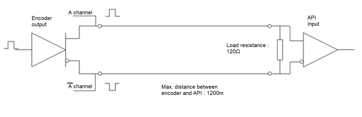
The RS422 and RS485 interfaces have been developed and perfected for high speed serial data transmission over long distances (up to 1200 meters) and are becoming more and more popular in the industrial sector and in particular in the transfer of encoder data.
Schematic diagram of an RS422 connection
Comparison table between RS422 and RS485
| PARAMETER | RS422 | RS485 | Unit |
| Number of driver and receivers | 1 Driver /10 Receivers | In bus, 32 receivers | |
| Theorical max. length of the connecting cable | 1200 | 1200 | Meters |
| Maximum transmission frequency | 10 | >10 | Mbps |
| Maximum voltage in common mode | ±7 | –7 to +12 | Volts |
| Differential driver output level | 2 ≤ |VOD| ≤ 10 | 1.5 ≤ |VOD| ≤ 5 | Volts |
| Ohmic load on 1 driver | ≥100 | ≥60 | Ω |
| Max. short-circuit current | 150 to GND | 250 to –7 V or 12 V | mA |
| Output off-voltage impedance | 60 | 12 | kΩ |
| Driver input impedance | 4 | 12 | kΩ |
| Receiver sensitivity (for a valid signal) | ±200 | ±200 | mV |
Screenshots
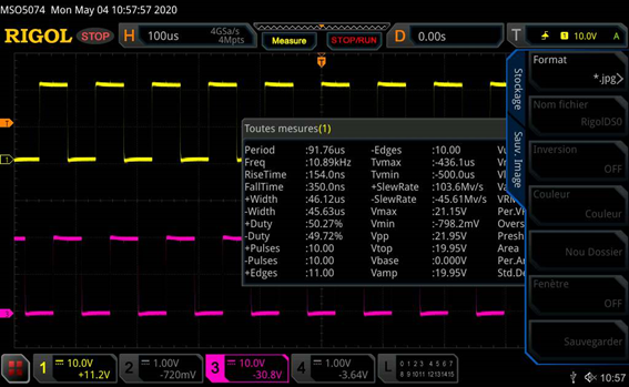
On the screenshot above we can see that for a power supply of 24 Volts and a cable length of one meter and a frequency of 10khz :
- The signal rise time is 154 ns
- The signal fall time is 350 ns
- The voltage drop caused by the output stage and the cable impedance of 1 meter and of (V Max) 21.15 V for a 24 Volts supply

After 10 meters of cable (screenshot above)
- The rise time (Rise Time) of the signal is 557 ns instead of 154 ns for 1 meter
- The signal fall time is 460 ns instead of 350 ns for 1 meter